CAMP

Greedy Dual Size (GDS) algorithm

Key Concepts:

1. Variable Size and Cost:
   • Unlike simple algorithms that treat all objects equally, GDS takes into account:
     • Size of the object (size(p)): Larger objects take up more space in memory.
     • Cost of the object (cost(p)): This can represent factors like time to retrieve the object, computational effort, or other resource usage.
2. Score H(p):
   • Each key-value pair ppp in the cache is assigned a score H(p). This score reflects the benefit of keeping the object in memory and is calculated using:
     • A global parameter L, which adjusts dynamically based on cache state.
     • The size(p) of the object.
     • The cost(p) associated with the object.
3. Eviction Strategy:
   • When the cache is full, and a new object needs to be added, GDS removes the object with the lowest score H(p). This process continues until there is enough space for the new object.

Proposition 1

L is non-decreasing over time.

• The global parameter L, which reflects the minimum priority H(p) among all key-value pairs in the KVS, will either stay the same or increase with each operation. This ensures stability and helps prioritize eviction decisions consistently.

For any key-value pair ppp in the KVS, the relationship holds:

L ≤ H(p) ≤ L + cost(p) / size(p)

• H(p), the priority of p, always lies between the global minimum L and L + cost(p) / size(p), ensuring H(p) reflects both its retrieval cost and size relative to other elements.

Intuition Behind Proposition 1:

• As L increases over time (reflecting the minimum H(p)), less recently used or less “valuable” pairs become increasingly likely to be evicted. This ensures that newer and higher-priority pairs stay in the KVS longer.

Key Insights from Proposition 1:

1. Delayed Eviction:
   • When p is requested again while in memory, its H(p) increases to L + cost(p) / size(p), delaying its eviction.
2. Impact of Cost-to-Size Ratio:
   • Pairs with higher cost(p) / size(p) stay longer in the KVS. For example, if one pair’s ratio is c times another’s, it will stay approximately c times longer.

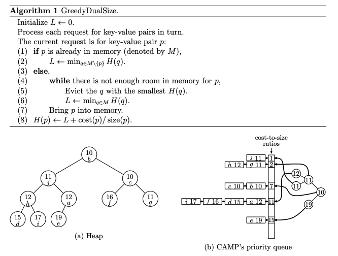
Key Points in the Diagram

1. Cost-to-Size Ratios:
   1. Key-value pairs are grouped into queues according to their cost-to-size ratio.
   2. Each queue corresponds to a specific cost-to-size ratio.
2. Grouping by Ratio:
   1. Within each queue, key-value pairs are managed using the Least Recently Used (LRU) strategy.
3. Priority Management:
   1. The priority (H-value) of a key-value pair is based on: H(p) = L + cost(p) / size(p)
      1. L: The global non-decreasing variable.
      2. cost(p) / size(p): The cost-to-size ratio of the key-value pair.
4. Efficient Eviction:
   1. CAMP maintains a heap that points to the head of each queue, storing the minimum H(p) from every queue.
   2. To identify the next key-value pair for eviction:
      1. The algorithm checks the heap to find the queue with the smallest H(p).
      2. It then evicts the key-value pair at the front of that queue (i.e., the least recently used pair in that cost-to-size group).

Rounding in CAMP

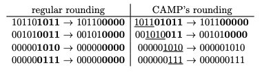
1. Purpose: To improve performance, CAMP reduces the number of LRU queues by grouping key-value pairs with similar cost-to-size ratios into the same queue.
2. Key Idea: Preserve the most significant bits proportional to the value’s size.

Proposition 2: Explanation of Rounding and Distinct Values

Implications

1. Trade-Off Between Precision and Efficiency:

   • A higher p preserves more precision but increases the number of distinct values (and thus computational complexity).

   • Lower p reduces the number of distinct values, making CAMP more efficient but less precise.

2. Rounding Efficiency:

   • By limiting the number of distinct values, CAMP minimizes the number of LRU queues, reducing overhead while still approximating GDS closely.

Proposition 3: Competitive Ratio of CAMP

Practical Implications

1. Precision ppp:

   • The smaller the ϵ (higher ppp), the closer CAMP approximates GDS.

   • For sufficiently large p, CAMP performs nearly as well as GDS.

2. Trade-off:

   • Higher p increases precision but also increases the number of distinct cost-to-size ratios and computational overhead.

CAMP’s Improvement Over GDS:

1. Approximation: CAMP simplifies H(p) by rounding the cost-to-size ratio, reducing the precision but making the algorithm more efficient.
2. Grouping: Key-value pairs are grouped by similar cost-to-size ratios, reducing the number of queues and simplifying priority management.
3. Tie-Breaking: CAMP uses LRU within each group to determine the eviction order, making it computationally cheaper.

Figure 4: Heap Node Visits

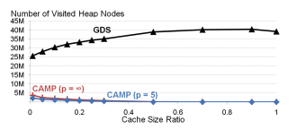
This figure compares the number of heap node visits for GDS and CAMP as a function of cache size:

1. GDS:

   • Heap size equals the total number of key-value pairs in the cache.

   • Every heap update (insertion, deletion, or priority change) requires visiting O(log⁡n) nodes, where n is the number of cache entries.

   • As cache size increases, GDS’s overhead grows significantly.

2. CAMP:

   • Heap size equals the number of non-empty LRU queues, which is much smaller than the total number of cache entries.

   • Heap updates occur only when:

     • The priority of the head of an LRU queue changes.

     • A new LRU queue is created.

   • As cache size increases, the number of non-empty LRU queues remains relatively constant, resulting in fewer heap updates.

Evaluation

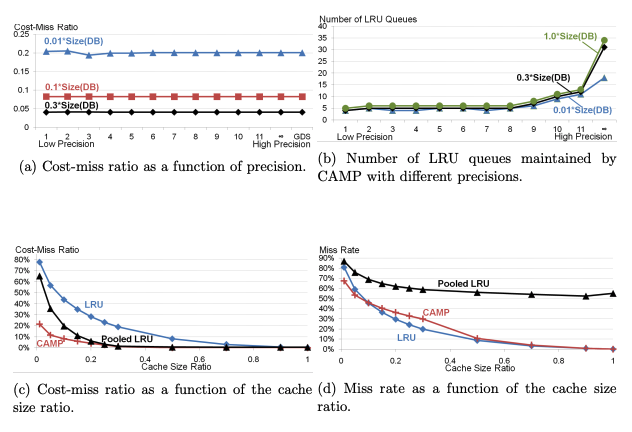
(a) Cost-Miss Ratio vs Precision

• 横轴：精度（Precision），从低到高。
• 纵轴：成本未命中比（Cost-Miss Ratio）。
• 结果：
  • 不同的缓存大小比（0.01、0.1 和 0.3）在较低精度下表现一致。
  • 提高精度后，成本未命中比没有显著变化。
  • 说明即使使用较低精度，CAMP 的成本未命中比也能接近 GDS（标准实现）。

(b) LRU Queues vs Precision

• 横轴：精度（Precision）。
• 纵轴：CAMP 维护的非空 LRU 队列数量。
• 结果：
  • 低精度（1-5）：CAMP 维持稳定的少量 LRU 队列（约 5 个）。
  • 高精度（>10）：队列数增加，尤其是在较大的缓存大小比（如 1.0）下。
  • 结论：
    • 在较低精度下，CAMP 能保持较低的计算开销，同时维持高效的队列管理。

(c) Cost-Miss Ratio vs Cache Size Ratio

• 横轴：缓存大小比（Cache Size Ratio），即缓存大小与 trace 文件中唯一键值对总大小的比值。
• 纵轴：成本未命中比（Cost-Miss Ratio）。
• 结果：
  • CAMP：
    • 在所有缓存大小下，成本未命中比最低。
    • 说明 CAMP 在高成本键值对管理上更具效率。
  • Pooled LRU：
    • 在较小缓存下表现稍差，但随着缓存增加，接近 CAMP。
  • LRU：
    • 成本未命中比始终最高。
  • 结论：
    • CAMP 优于 LRU 和 Pooled LRU，尤其是在小缓存下。

(d) Miss Rate vs Cache Size Ratio

• 横轴：缓存大小比（Cache Size Ratio）。
• 纵轴：未命中率（Miss Rate）。
• 结果：
  • CAMP：
    • 未命中率显著低于 LRU 和 Pooled LRU，尤其在小缓存下表现最优。
  • Pooled LRU：
    • 未命中率随着缓存增大而下降，但始终高于 CAMP。
    • 最低成本池（cheapest pool）未命中率接近 100%，次低成本池未命中率达到 65%。
  • LRU：
    • 始终高于 CAMP 和 Pooled LRU。
  • 结论：
    • CAMP 在多种缓存大小下都保持较低的未命中率，且比 Pooled LRU 更均衡。

CAMP 的适应能力：访问模式变化的分析

实验设置：

• 使用 10 个不同的 trace 文件，每个文件包含 400 万个键值对引用。
• 每个 trace 文件（如 TF1、TF2 等）中的请求在其结束后不会再被引用，模拟访问模式的突然变化。
• 访问模式具有倾斜分布（如 Zipf 分布），每个 trace 文件中的高成本对象可能在下一次访问中完全无效。

目标：

• 比较 CAMP、Pooled LRU 和 LRU 在不同缓存大小下对访问模式突变的适应能力。
• 评估三种算法在突然变化后清除旧的高成本键值对的效率，以及对总体性能（如成本未命中比和未命中率）的影响。

不同算法的行为分析

1. LRU：

   • 按最近使用排序，当新请求的总大小超过缓存大小时清除旧数据。

   • 当缓存大小比为 1 时，清除 TF1 数据的时间点对应于 TF3 开始请求的第一个键值对。

2. Pooled LRU：

   • 将键值对按成本分组，每组分配固定比例的缓存空间。

   • 高成本池占据 99% 的缓存空间，因此在每个新 trace 开始时会突然清除一批旧数据。

   • 对于缓存大小比 2/3 或更高的情况，直到 TF4（约 800 万请求后）才会清除所有 TF1 数据。

3. CAMP：

   • 对每个成本-大小比维护 LRU 队列，这些队列的大小可以动态调整。

   • 优先淘汰较低优先级的数据，但高成本数据即使来自旧 trace，也具有一定保留优先级。

   • 当新数据的总大小超过缓存时，旧 trace 的高成本数据才会被逐步清除。

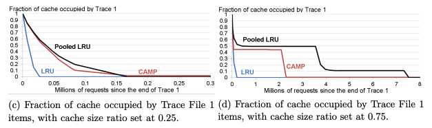
图 6c：缓存比 0.25（小缓存）

1. LRU：

   • 清除最快，仅需 2.1 万次请求 即完全清除 Trace 1 的所有键值对。

   • 由于 LRU 优先淘汰最久未使用的数据，小缓存下表现最佳。

2. Pooled LRU：

   • 清除速度较慢，需要 13.1 万次请求。

   • 原因：Pooled LRU 按成本对键值对分组，高成本池占用较多缓存空间，导致清除滞后。

3. CAMP：

   • 初期清除速度比 Pooled LRU 更快，但最后完全清除所有键值对需到 TF3 结束（770 万次请求）。

   • 然而，这些未被清除的 Trace 1 数据仅占缓存的 2%，说明 CAMP 优先保留了高成本键值对。

图 6d：缓存比 0.75（大缓存）

1. LRU：

   • 同样清除最快，几乎在 Trace 2 开始时就清除掉大部分 Trace 1 的数据。

   • 说明即使缓存较大，LRU 仍然倾向淘汰旧数据。

2. Pooled LRU：

   • 清除延迟显著，需要 730 万次请求，接近 TF3 结束。

   • 原因：高成本池占用过多缓存空间，延迟清除低成本和无用数据。

3. CAMP：

   • 大部分 Trace 1 数据在较早阶段被淘汰，仅保留少量最昂贵的键值对（占缓存比小于 0.6%）。

   • 即使在 4000 万次请求后，这些高成本键值对仍在缓存中，但对整体缓存利用影响极小。

针对不同大小但成本相同的键值对，CAMP 优先保留较小的键值对，从而降低未命中率和成本未命中比。

针对相同大小但成本不同的键值对，CAMP 优先保留高成本键值对，在成本未命中比上显著优于其他算法。

与其他算法的对比：

• LRU：适用于简单场景，但无法处理成本差异。

• Pooled LRU：小缓存情况下表现不错，但静态分区策略限制了其大缓存场景的效率。

CAMP 的适应性：在处理多样化的成本分布时，通过动态调整和四舍五入策略，CAMP 在复杂负载下表现出更高的灵活性和效率。

Questions

What is the time complexity of LRU to select a victim?

O(1) because the least recently used item is always at the tail of the list.

What is the time complexity of CAMP to select a victim?

O(logk) CAMP identifies the key-value pair with the smallest priority from the heap, deletes it and then heapifies.

Why does CAMP do rounding using the high order bits?

• CAMP rounds cost-to-size ratios to reduce the number of distinct ratios (or LRU queues).
• High-order bits are retained because they represent the most significant portion of the value, ensuring that approximate prioritization is maintained.

How does BG generate social networking actions that are always valid?

Pre-Validation of Actions:

• Before generating an action, BG checks the current state of the database to ensure the action is valid. For instance:
  • A friend request is only generated if the two users are not already friends or in a “pending” relationship.
  • A comment can only be posted on a resource if the resource exists.

Avoiding Concurrent Modifications:

• BG prevents multiple threads from concurrently modifying the same user’s state.

How does BG scale to a large number of nodes?

BG employs a shared-nothing architecture with the following mechanisms to scale effectively:

1. Partitioning Members and Resources:

   • BGCoord partitions the database into logical fragments, each containing a unique subset of members, their resources, and relationships.

   • These fragments are assigned to individual BGClients.

2. Multiple BGClients:

   • Each BGClient operates independently, generating workloads for its assigned logical fragment.

   • By running multiple BGClients in parallel across different nodes, BG can scale horizontally to handle millions of requests.

3. D-Zipfian Distribution:

   • To ensure realistic and scalable workloads, BG uses a decentralized Zipfian distribution (D-Zipfian) that dynamically assigns requests to BGClients based on node performance.

   • Faster nodes receive a larger share of the logical fragments, ensuring even workload distribution.

4. Concurrency Control:

   • BG prevents simultaneous threads from issuing actions for the same user, maintaining the integrity of modeled user interactions and avoiding resource contention.

True or False: BG quantifies the amount of unpredictable data produced by a data store?

True.

This is achieved through:

• Validation Phase:
  • BG uses read and write log records to detect instances where a read operation observes a value outside the acceptable range, classifying it as “unpredictable data.”
• Metrics Collection:
  • The percentage of requests that observe unpredictable data (τ) is a key metric used to evaluate the data store’s consistency.

How is BG’s SoAR different than its Socialites rating?

SoAR (Social Action Rating): Represents the maximum throughput (actions per second) a data store can achieve while meeting a given SLA.

Socialites Rating: Represents the maximum number of concurrent threads (users) a data store can support while meeting the SLA.

Reference: https://citeseerx.ist.psu.edu/document?repid=rep1&type=pdf&doi=d6f9678772a09ca29101f5efce583960ecf53745